Estimation of Time of Death

Last updated: November 10, 2024

Overview

The determination of the time of death or post-mortem interval (time elapsed since death) is important in criminal and civil situations as it can tell us when a crime was committed. Unfortunately, all of the methods being currently used cannot be fully relied on as they are not completely accurate.

Apart from post-mortem changes already discussed there are other methods to estimate time of death.

Temperature gauge

The human body cools after death as when one dies, the metabolic production and circulation of heat ceases.

  • Assumptions made to measure PMI using temperature
    • Body temperature at death was normal at 37°C
    • Body cooling follows a predictive pattern that allows one to project what the prior temperature was
  • Multiple factors affect this
    • Ambient temperature – the greater the difference between body temperature and environmental temperature the faster the cooling.
    • Clothing – heavily clothed bodies will cool slower
    • Body size – the bigger the surface area of the body relative to mass the faster the cooling
    • Air movement – windy conditions cause faster cooling
    • Exposure to water
    • Thermal conductivity of surface the body is on

Core temperature is measured rectally as this is more accurate. Serial measurements are taken which are plotted on a graph against time. If one assumes the body temperature was 37°C at the time of death that means then finding the point on this section corresponding to the measured rectal temperature should allow extrapolation back to the 37°C point which is at zero on the time scale, thus giving the PMI.

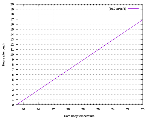
Another way of estimating PMI using temperature is the use of formulas:

The Glaister equation:

  • Celsius version (36.9°C – rectal temperature in °C) * 6/5
  • Fahrenheit version 98.4°F – rectal temperature in Fahrenheit/ 1.5
A graphical representation of the Glaister equation with values from 37°C to 20°C (commonly used as ambient temperature)

Chemical changes in body fluids

Quantifying the level of potassium in vitreous humour is a reliable way of determining PMI. Any factor that increases the rate of decomposition such as hot temperatures will also cause an increase in potassium levels.

  • Advantages
    • Easily accessible to the pathologist
    • Protected from bacterial contamination owing to its location
  • Disadvantages
    • Loses accuracy after a few days post-mortem as volume changes due to decomposition
    • Subject to pre-analytical, analytical and post-analytical errors hence has a high chance of being innaccurate

Gastric emptying

Trying to determine the time interval between eating and the time of death can be used to determine PMI. If one can ascertain when the deceased last ate then you can estimate PMI.

A small meal takes 1-3 hours to digest while a medium sized meal takes 3-4 hours. A large meal takes 4-6 hours approximately

Forensic entomology

Another tool that can be used in determining PMI is insect activity on the body. Just as in life, dead human tissues attract a wide array of insects. Knowledge of the different species and the rate of development can help determine when a person died.

Scene markers

Objects found at the scene can be used to estimate PMI. They include:

  • Uncollected mail or newspapers.
  • Whether the lights are on or off
  • A TV schedule opened to a time and date.
  • How the individual is dressed.
  • Any food that is out or dirty dishes in the sink.
  • Sales receipts or dated slips of paper in the deceased’s pockets.
  • When the neighbours last saw the individual or observed a change in his habits.

Henssge’s normogram

This involves the use of a nomogram to estimate the time of death. There is a 95% chance of the time falling within the correct range

  • Adjustments for the following are built in:
    • Body weight
    • Ambient temperature
    • Dry or wet clothing
    • Still or moving air
    • Still or moving water
  • Disadvantages
    • Unable to test the strength of the variables
    • Does not allow the variation of the variables over time
Reference Intervals
Biochemistry
ACTHP: <80 ng/L
ALTP: 5–35 U/L
AlbuminP: 35–50 g/L
AldosteroneP: 100–500 pmol/L
Alk. phosphataseP: 30–130 U/L
α-AmylaseP: 0–180 IU/dL
α-FetoproteinS: <10 kU/L
Angiotensin IIP: 5–35 pmol/L
ADHP: 0.9–4.6 pmol/L
ASTP: 5–35 U/L
BicarbonateP: 24–30 mmol/L
BilirubinP: 3–17 μmol/L
BNPP: <50 ng/L
CRPP: <10 mg/L
CalcitoninP: <0.1 mcg/L
Calcium (ionized)P: 1.0–1.25 mmol/L
Calcium (total)P: 2.12–2.60 mmol/L
ChlorideP: 95–105 mmol/L
CholesterolP: <5.0 mmol/L
VLDLP: 0.128–0.645 mmol/L
LDLP: <2.0 mmol/L
HDLP: 0.9–1.93 mmol/L
Cortisol AMP: 450–700 nmol/L
Cortisol MidnightP: 80–280 nmol/L
CK ♂P: 25–195 U/L
CK ♀P: 25–170 U/L
CreatinineP: 70–100 μmol/L
FerritinP: 12–200 mcg/L
FolateS: 2.1 mcg/L
FSHP: 2–8 U/L ♂; >25 menopause
GGT ♂P: 11–51 U/L
GGT ♀P: 7–33 U/L
Glucose (fasting)P: 3.5–5.5 mmol/L
Growth hormoneP: <20 mu/L
HbA1C (DCCT)B: 4–6%
HbA1C (IFCC)B: 20–42 mmol/mol
Iron ♂S: 14–31 μmol/L
Iron ♀S: 11–30 μmol/L
Lactate (venous)P: 0.6–2.4 mmol/L
Lactate (arterial)P: 0.6–1.8 mmol/L
LDHP: 70–250 U/L
LHP: 3–16 U/L
MagnesiumP: 0.75–1.05 mmol/L
OsmolalityP: 278–305 mosmol/kg
PTHP: 0.8–8.5 pmol/L
PotassiumP: 3.5–5.3 mmol/L
Prolactin ♂P: <450 U/L
Prolactin ♀P: <600 U/L
PSAP: 0–4 mcg/mL
Protein (total)P: 60–80 g/L
Red cell folateB: 0.36–1.44 μmol/L
Renin (erect)P: 2.8–4.5 pmol/mL/h
Renin (recumbent)P: 1.1–2.7 pmol/mL/h
SodiumP: 135–145 mmol/L
TBGP: 7–17 mg/L
TSHP: 0.5–4.2 mU/L
T4P: 70–140 nmol/L
Free T4P: 9–22 pmol/L
TIBCS: 54–75 μmol/L
TriglyceridesP: 0.50–2.3 mmol/L
T3P: 1.2–3.0 nmol/L
Troponin TP: <0.1 mcg/L
Urate ♂P: 210–480 μmol/L
Urate ♀P: 150–390 μmol/L
UreaP: 2.5–6.7 mmol/L
Vitamin B12S: 0.13–0.68 nmol/L
Vitamin DS: 50 nmol/L
Arterial Blood Gases
pH7.35–7.45
PaCO₂4.7–6.0 kPa
PaO₂>10.6 kPa
Base excess±2 mmol/L
Urine
Cortisol (free)<280 nmol/24h
Hydroxyindole acetic acid16–73 μmol/24h
Hydroxymethylmandelic acid16–48 μmol/24h
Metanephrines0.03–0.69 μmol/mmol cr.
Osmolality350–1000 mosmol/kg
17-Oxogenic steroids ♂28–30 μmol/24h
17-Oxogenic steroids ♀21–66 μmol/24h
17-Oxosteroids ♂17–76 μmol/24h
17-Oxosteroids ♀14–59 μmol/24h
Phosphate (inorganic)15–50 mmol/24h
Potassium14–120 mmol/24h
Protein<150 mg/24h
Protein/creatinine ratio<3 mg/mmol
Sodium100–250 mmol/24h
Haematology
WCC4.0–11.0 ×10⁹/L
RBC ♂4.5–6.5 ×10¹²/L
RBC ♀3.9–5.6 ×10¹²/L
Hb ♂130–180 g/L
Hb ♀115–160 g/L
PCV ♂0.4–0.54 L/L
PCV ♀0.37–0.47 L/L
MCV76–96 fL
MCH27–32 pg
MCHC300–360 g/L
RDW11.6–14.6%
Neutrophils2.0–7.5 ×10⁹/L (40–75%)
Lymphocytes1.0–4.5 ×10⁹/L (20–45%)
Eosinophils0.04–0.44 ×10⁹/L (1–6%)
Basophils0–0.10 ×10⁹/L (0–1%)
Monocytes0.2–0.8 ×10⁹/L (2–10%)
Platelets150–400 ×10⁹/L
Reticulocytes0.8–2.0% / 25–100 ×10⁹/L
Prothrombin time10–14 s
APTT35–45 s
Paediatric
Pulse Rate (bpm)
Neonate140–160
Infant <1yr120–140
1–5 years110–130
5–12 years80–120
>12 years70–100
Respiratory Rate (tachypnoea)
0–2 months≥60/min
2–12 months≥50/min
1–5 years≥40/min
>5 years≥30/min
Blood Pressure (mmHg)
Term65/45
1 year75/50
4 years85/60
8 years95/65
10 years100/70
Weight Formulas
3–12 months(a + 9)/2 kg
1–6 years2a + 8 kg
>6 years(7a − 5)/2 kg
Haemoglobin (g/dL)
Term newborn13–20
1 month11–18
2 months10–15
1–2 years10–13
>2 years11–14
MUAC (6 months–5 years)
Obese>17.5 cm
Normal13.5–17.4 cm
At risk12.5–13.4 cm
Moderate malnutrition11.5–12.4 cm
Severe malnutrition<11.5 cm
Developmental Milestones
Social smile1.5 months
Head control4 months
Sits unsupported7 months
Crawls10 months
Stands unsupported10–12 months
Walks12–13 months
Talks18 months
CSF WBC (/mm³)
Term newborn0–25
>2 weeks0–5
Calculator

Post Discussion

Your email address will not be published. Required fields are marked *